
Companion to Why does the plan keep changing? · September 15, 2026
About the article
The article combines established planning research, recent simulation studies, two documented details from Brandon's work, and a new synthetic calculation. Its interpretation is that revisions should be diagnosed by their cause and evaluated against the specific commitments they disturb. It does not claim to invent selective freezing, rescheduling penalties, or forecast evolution models.
The research search was targeted, not a systematic literature review. Recent primary studies were checked alongside foundational work needed to avoid presenting established ideas as new. Publication and version dates were checked against September 15, 2026. No recommendation depends on an unverified future publication.
Sources used in the article
1. Blackburn, Kropp and Millen — 1986
A Comparison of Strategies to Dampen Nervousness in MRP Systems. Management Science 32(4), 413–429. April 1986. Publisher and abstract.
Basis read: publisher abstract. The study isolates interaction between lot sizing and the planning horizon; demand, supply and lead-time uncertainty are excluded. The article uses that narrow finding to establish that rescheduling can have an internal source. It does not extrapolate a universally best freeze length.
2. Weijers and colleagues — 2025
Improving Plan Stability in Semiconductor Manufacturing Through Stochastic Optimization: A Case Study. 2025 Winter Simulation Conference. Full proceedings paper.
Basis read: full paper. Company-derived data and an aggregated simulation; selected high-demand products, excluding ramp-up and ramp-down. Supply uncertainty is outside the study. Alternative optima are a mechanism described by the authors; this does not imply a deterministic solver randomly changes its answer on identical inputs. Stability and operating performance are simulation results, not measured deployment benefits.
3. Meistering and Stadtler — 2019 / 2020
Stabilized-cycle strategy for a multi-item, capacitated, hierarchical production planning problem in rolling schedules. Online January 29, 2019; Business Research volume 13, 2020. Full paper.
Basis read: full paper, especially detailed scheduling and experimental design. Six products on one machine in 16 instances; setup times are omitted. Setup timing can remain fixed while daily quantities change. Service-based reopening is part of the strategy. Its cost and service results do not dominate every comparator on every measure.
4. Abay, Kaihara and Kokuryo — May 2026
Stochastic Multi-Objective Sales and Operations Planning with Plan Stability Objectives and Supply Order Allocation Using Simulation–Optimization. International Journal of Automation Technology 20(3), 189–206; May 5, 2026. Full paper.
Basis read: full paper, frozen-horizon rules and sensitivity analysis. Vehicle-assembly simulation with uncertain imported supply. Different nervousness measures move differently. Because the experimental horizons and customer-patience assumptions change together, it cannot isolate the causal effect of calendar freeze length. Its preferred model setting is not a transferable prescription.
5. Schlenkrich, Seiringer, Altendorfer and Parragh — August 2026 version
Enhancing Rolling Horizon Production Planning Through Stochastic Optimization Evaluated by Means of Simulation. arXiv:2402.14506, version 3, August 11, 2026; first submitted February 2024. Preprint. Full v3 · Version history.
Basis read: full v3. The physical execution freeze is one period. A separate non-anticipativity parameter makes early decisions equal across scenarios within a solve; that does not guarantee unchanged decisions in subsequent replans. Initial inventory buffers in the optimization cases differ from MRP's maintained safety stock. The article omits headline savings comparisons, some of which involve different service levels.
6. Forel and Grunow — 2022 / 2023
Dynamic stochastic lot sizing with forecast evolution in rolling-horizon planning. First online September 19, 2022; Production and Operations Management, 2023. Publisher paper.
Basis read: paper, numerical studies and limitations. Historical forecast information, synthetic and real inputs, and rolling out-of-sample simulation support conditional value from future adaptation. Better statistical fit can still yield worse decisions under misspecification. No percentage from the study is presented as Brandon's result or as an expected gain for another business.
Operating examples
The operating examples are accounts of Brandon’s professional work, distinct from Allelon Working Collaborative client results. The 617 archived files describe overlapping planning periods, not 617 independent observations. No measured benefit from the 72-hour freeze is claimed. The distinction between an event's occurrence, discovery, and receipt by planning is diagnostic guidance; no proportions of revision causes are asserted.
Reproducing the six-job illustration
Files: Python source, JSON inputs and sensitivity results, comparison CSV, PNG figure, SVG figure.
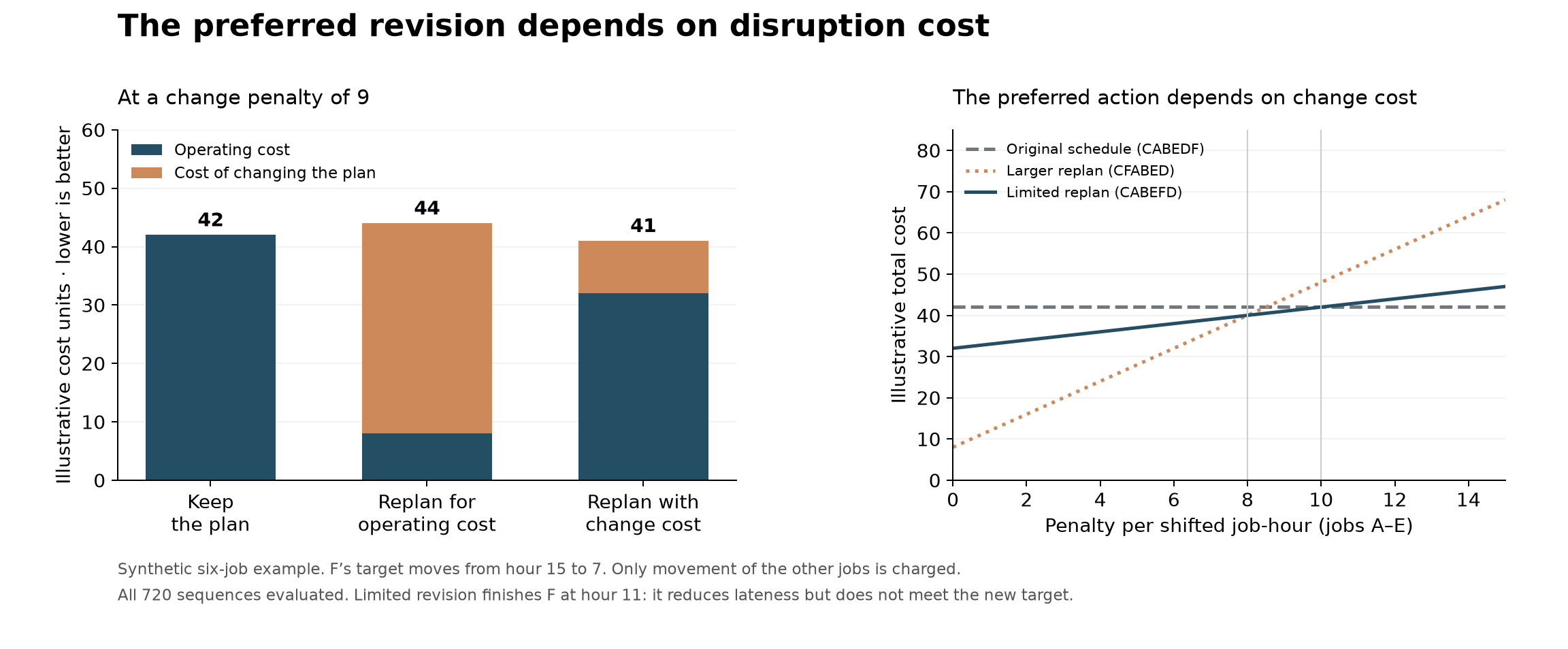
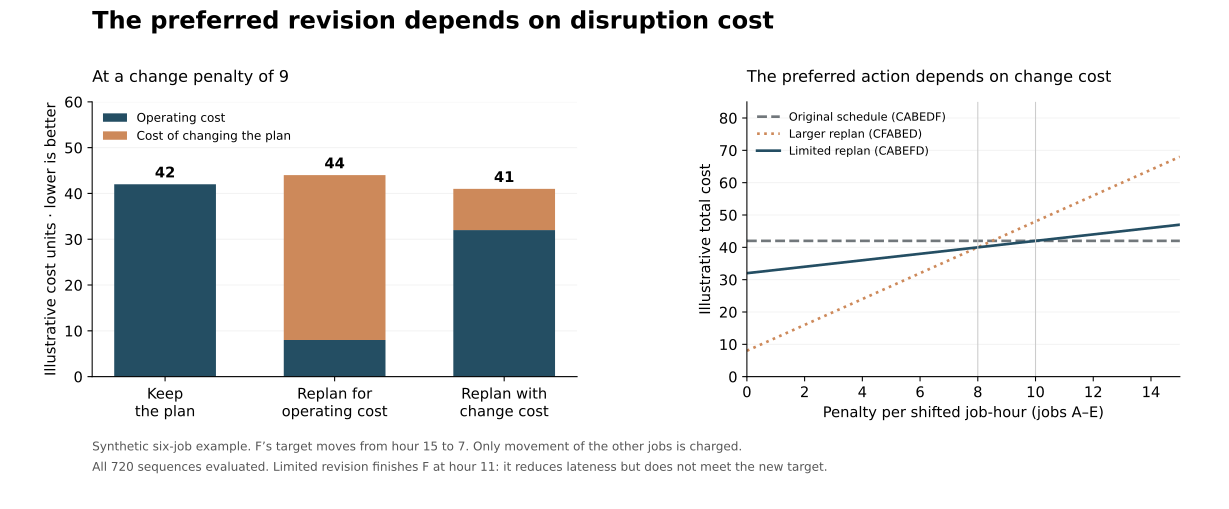
Run python3 freeze_analysis.py in a directory containing the source to regenerate the JSON and CSV. The calculation uses only Python's standard library. Add --plot with Matplotlib installed to regenerate both figures. Verification here used Python 3.14.6 and Matplotlib 3.11.2.
Inputs and assumptions
One machine, six jobs, all available at time zero. Every sequence starts as early as possible; intentional idling is excluded. Jobs cannot be interrupted. All replanning occurs before processing begins. Time is measured in hours from that common starting point.
| Job | Processing hours | Family | Original due hour | Lateness cost per hour |
|---|---|---|---|---|
| A | 2 | X | 5 | 4 |
| B | 3 | X | 8 | 3 |
| C | 1 | Y | 6 | 5 |
| D | 2 | Y | 12 | 2 |
| E | 2 | X | 10 | 4 |
| F | 1 | Y | 15 | 6 |
Changing families takes one hour and costs three illustrative units. No initial setup is charged. There is no earliness penalty. Due dates are soft: lateness incurs a cost, so a schedule with late jobs remains feasible. F's due hour changes from 15 to 7; all other inputs remain fixed.
Operating cost is the sum of weighted positive lateness plus family-change costs. The original optimal sequence under the old due dates is C–A–B–E–D–F, with operating cost 6. After the due-date update, its operating cost becomes 42.
Disruption is the sum, across jobs A–E, of the absolute difference between proposed and original start times. F's own requested advancement is excluded. These are job-hours moved, not machine downtime. The linear penalty is a transparent illustration of coordination cost; it is not an empirical cost model.
Total cost = operating cost + change penalty × job-hours moved.
At a penalty of nine, the unrestricted operating-cost optimum C–F–A–B–E–D shifts the other jobs' starts by four job-hours: 8 + 9 × 4 = 44. The total-cost optimum C–A–B–E–F–D shifts them by one job-hour: 32 + 9 × 1 = 41. Holding the original sequence costs 42.
F finishes at hour 2 in the larger revision, hour 11 in the limited revision, and hour 13 if the plan is held. The latter two miss the new hour-7 target by four and six hours respectively. A hard hour-7 deadline would eliminate those alternatives.
Checks and sensitivity
All 720 permutations are enumerated. Every result is checked for unique jobs, nonoverlapping processing, the required intervening setup time, and independently recomputed weighted lateness. The original optimum and the selected penalty-six, penalty-nine and penalty-twelve results have explicit assertions. A 1,501-point sweep evaluates the optimum at penalties from 0 to 15 in steps of 0.01. A separate review enumerated all sequences to confirm the three regimes and their boundaries.
At penalties 6, 9, and 12, the winning sequences are respectively C–F–A–B–E–D, C–A–B–E–F–D, and C–A–B–E–D–F. The larger revision wins strictly between 0 and 8; larger and limited tie at 8; limited wins between 8 and 10; limited and unchanged tie at 10; unchanged wins above 10. Ties use least movement, then alphabetical sequence; the original-plan tie uses alphabetical sequence. The chart's right panel displays the three fixed schedules, not three different algorithms being rerun at each plotted point.
The example has no material shortages, hard deadlines, qualification rules, uncertain processing, failures, strategic rush orders, or later arrivals. It does not model repeated replanning or estimate a calendar freeze. Its small one-unit advantage for limited revision at the main penalty is deliberately reported as fragile.